
C2.Q1 Fit a model relating birth mass to maternal dominance status (n.b., dominance status is a variable in the unicorns dataset; it is described in table 2.2 of Using R, but we have not made much use of it yet).
This will involve fitting a linear model, very similar to that we’ve already considered in detail using maternal age at parity as the predictor variable:
# fit the model
m<-lm(BirthWt~dominance, data=unicorns)
summary(m)$coefficients
## Estimate Std. Error t value Pr(>|t|)
## (Intercept) 2.0746426 0.05959653 34.811464 9.196846e-177
## dominance 0.2868031 0.09195838 3.118836 1.865509e-03The question was a bit open-ended. It didn’t say what you should get out of this model. The most interesting thing is probably the slope, which seems to indicate that females with higher dominance status have heavier babies.
C2.Q2 Write a formal description of the model you just fitted.
I fitted a model of offspring birth mass (


where 


I’ve stressed that units are critical to model description. But sometimes the way we measure things in real biological data collection scenarios is a bit inconvenient for succinctly describing units. Dominance is measured as a proportion, and proportions are unitless (this one has number of individuals – to which the mother is dominant – in the numerator, and number of individuals – in the population – in the denominator, so they cancel out). But describing the units of the regression slope as kg, which in a sense it is, is just asking for your reader to be confused. More fully described, the units are kg of offspring birth mass difference between an individual with a dominance score of zero, and a female with a dominance score of 1. However, fully writing out “kg difference between females that are not dominant to any others and those that are dominant to all others’’ does not make for silken prose. In this situation, you need to make very clear to explain all the units (of both the measured quantity and any regression terms) at least once. If after that you give some unitless numbers, you are not committing too great a sin.
C2.Q3 Write a sentence or two describing what you take to be the key result of this model.
Offspring birth mass increases with maternal dominance status, with a change of 0.29 kg (SE: 0.29) between females that are not dominant to any others and those that are dominant to all others.
C2.Q4 Make a visualisation of the your model’s results.
This is closely analogous to figure :
# put the raw data in the background
plot(unicorns$dominance,unicorns$BirthWt,
     xlab="Maternal dominance status (proportion)",
     ylab="Offspring birth mass (kg)", col="gray")
# a range over which to show predictions
domRange<-seq(min(unicorns$dominance),
     max(unicorns$dominance),length.out=30)
# our custom function to add a prediction line,
# with associated prediction intervals
predInterval(m,data.frame(dominance=domRange))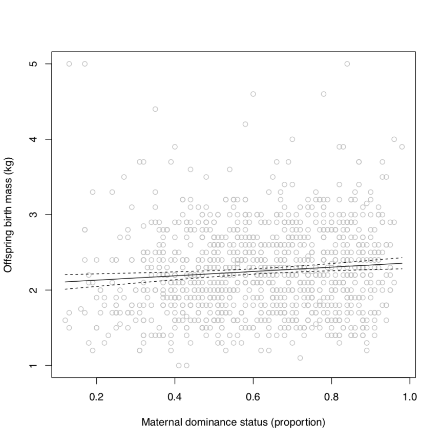
Figure 1. The relationship between offspring birth mass and maternal dominance status (proportion of extant females to which each focal individual’s mother was dominant) in unicorns (Monoceros europus). The solid line depicts the fitted regression and the dashed lines represent the 95% confidence intervals of predictions.
Remember that the caption is a critical part of any figure! It simply is not a scientific figure without descriptive caption. Note that I did not elaborate on units in the caption, beyond those aspects that were already clear from the descriptors that I chose to use in the plot’s axis labels.
C2.Q5 Which do you think is more important to offspring birth mass: maternal age or maternal dominance status?
Here are the coefficients for comparable simple regression models for the two predictor variables:
# the model fitted in chapter 2
summary(mMatAge)$coefficients
## Estimate Std. Error t value Pr(>|t|)
## (Intercept) 2.01193964 0.040634103 49.513573 5.417337e-276
## MumAge 0.04667381 0.007128639 6.547366 9.176103e-11# the model fitted to answer question 1
round(summary(m)$coefficients,4)## Estimate Std. Error t value Pr(>|t|)
## (Intercept) 2.0746 0.0596 34.8115 0.0000
## dominance 0.2868 0.0920 3.1188 0.0019You would have to be forgiven if you thought that the bigger number for the effect of dominance on birth mass meant it had a larger effect. You’d be forgiven, but wrong. A straight-up comparison is not possible, because the regression coefficients are in different units. The smaller value of 0.047 has its effect across a much larger range of values (ages 1 to 13) than the dominance effect (values of zero to one). We can use our regressions to calculate the difference in expected birth mass from smallish to largish values of each predictor variable in turn. A range of maternal ages that might be informative (discounting the very oldest ages to which very few unicorns survive) might be from ages 1 to 10:
# maternal age model coefficients
co_age<-coef(mMatAge)
# informative range of age
ageVals<-c(1,10)
# predictions
co_age[1]+co_age[2]*ageVals
## [1] 2.058613 2.478678From the figure we just made, we can see that a sensible range of dominance values ranges from about 0.2 to essentially 1.0:
# maternal age model coefficients
co_dom<-coef(m)
# informative range of age
domVals<-c(0.2,1.0)
# predictions
co_dom[1]+co_dom[2]*domVals
## [1] 2.132003 2.361446So, both predictor variables seem to drive changes of broadly similar magnitude. If one is more important, is is probably maternal age. Across the bulk of the span of maternal age in the data, there is a slightly larger range of expected offspring birth masses.
