End of chapter questions for elementary statistical modelling, chapter 7

C7.Q1 Conduct and report on an analysis of the overall shape of the relationship between birth mass and maternal dominance status. Your answer should reflect different elements of (i) fitting a model using R, (ii) properly describing your model, and (iii) making a clear and complete biological statement of your findings.

I investigated potential non-linearities in the regression of offspring birth mass ( $m_i$ ) on maternal dominance status ( $d_i$ ) of individual ( $I$ ) unicorns using a polynomial regression approach described by
$m_i = \alpha + \left( \Sigma_{j=1}^k \beta_jd_i^j \right) + e_i$ ,
where $\alpha$ is the model intercept and $e_i$ are residuals. $\beta_j$ is a polynomial regression term of order $j$ and $k$ is the order of the polynomial regression. I considered value of $k=1$ (linear regression), $k=2$ (quadratic regression) and $k=3$ (cubic regression).

The polynomial regressions were implemented with the following code:

m1<-lm(BirthWt~dominance, data=unicorns)
m2<-lm(BirthWt~poly(dominance,order=2,raw=TRUE), 
     data=unicorns)
m3<-lm(BirthWt~poly(dominance,order=3,raw=TRUE), 
     data=unicorns)

I evaluated the models visually by plotting

domRange<-seq(min(unicorns$dominance),
     max(unicorns$dominance),length.out=30)
par(mfrow=c(1,3))
plot(unicorns$dominance,unicorns$BirthWt,col="gray")
predInterval(m1,data.frame(dominance=domRange))
mtext(side=3,outer=FALSE,"first order")
plot(unicorns$dominance,unicorns$BirthWt,col="gray")
predInterval(m2,data.frame(dominance=domRange))
mtext(side=3,outer=FALSE,"second order")
plot(unicorns$dominance,unicorns$BirthWt,col="gray")
predInterval(m3,data.frame(dominance=domRange))
mtext(side=3,outer=FALSE,"third order")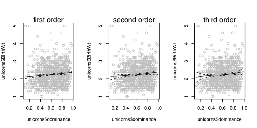

Figure 1. Depictions of first- through third-order polynomial regressions of birth mass (kg) on maternal dominance status (proportion of extant individuals to which a focal individual’s mother is dominant) in unicorns.

There appears to be very little evidence for non-linear components of the regression of offspring birth mass on maternal dominance status (figure 1).

Note that this answer could be further elaborated. Did your answer include a higher quality figure? If so, how was it better? Mine could use sub-plot labels, nicer axis labels giving units, and its caption could more completely describe what the solid and dashed lines are. My description could benefit from some quantitative description of the estimated coefficients of the polynomial regression models. Unless I had a very specific reason to be interested in curvature (rather than the perfectly reasonable motivation of simply checking whether there is any major curvature that I might want to be aware of), I would be inclined to focus any quantitative reporting on the linear regression model.

You may have noticed a change in my model description strategy. I changed from my standard use of $y$ for a response variable, to one that is a little more tailored to the data at hand, using $m$ instead for birth mass. In the middle of any given document, you would absolutely want to avoid making any such change. My purpose in changing is to avoid the impression that $y$ is somehow special for describing response variables. So long as your description is complete, virtually any symbols can be sensible. Avoid using terms that could easily lead to misunderstanding. For example, even if some variable might make sense to denote $e$ , don’t. $e$ (or sometimes $\epsilon$ for the Greek letter “epsilon’’) is so commonly used for residuals, that using them for other purposes will normally be unfortunate.

C7.Q2 Make up a bit of code that can plot the function relating to an arbitrary polynomial over some range of values.

Here is my function. The key argument is terms, which is assumed to be the terms of the model, starting with the intercept, then the linear term, then a quadratic term, going on up to however high of a polynomial order is desired. The other argument, xvals, has a default, so if we don’t specify values of $x$ over which to plot when using this function, it will plot over a range from zero to ten:

myPoly<-function(terms,xvals=seq(0,10,length.out=30)){
  k<-length(terms)-1
  n<-length(xvals)
  yvals<-array(dim=n)
  for(i in 1:n){
    yvals[i]<-sum(terms*xvals[i]^(0:k))
  }
  plot(xvals,yvals,type="l")
}
# test the function
par(mfrow=c(1,2))
myPoly(c(0,1))
myPoly(c(0,5,-1))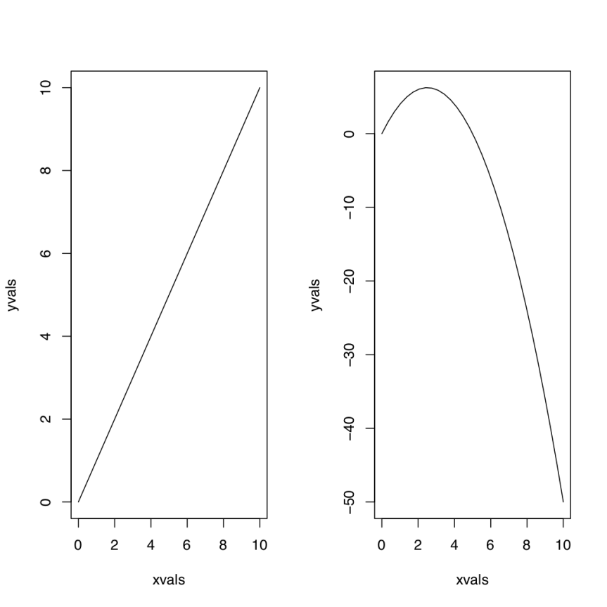

unnamed-chunk-27-1 You should be able to follow how my function worked, by taking it one line at a time. It may help you if I break down one key part. In order to raise some number (say, 2), to the powers zero through 3, a compact trick is

2^(0:3)

## [1] 1 2 4 8

C7.Q3 Use your function to work out (probably by trial and error, but think it through first if you can!) how to make a function that initially increases quickly, then slows down (though perhaps still increases, just slowly), and then begins to increase quickly again.

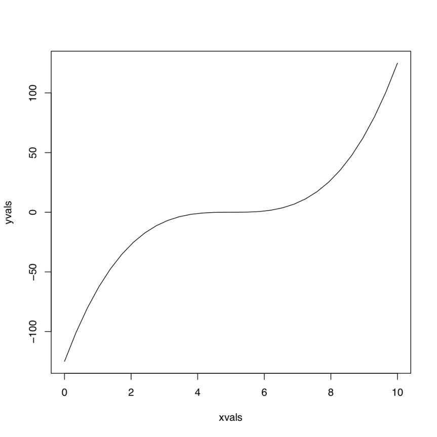
The simplest function is a pure cubic function according to $y = x^3$ , but whether it has the qualities described in the question depends on the range of values of which it is evaluated. Over ranges spanning zero, it works.

myPoly(c(0,0,0,1),xvals=seq(-3,3,length.out=30))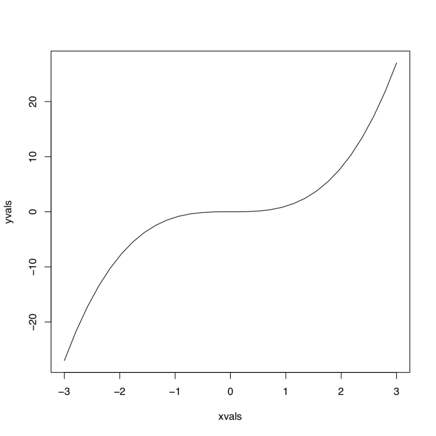

unnamed-chunk-29-1

If we had wanted the function to work over the original range that was the default for the function we made in the last question, we would have to shift it to the right. This takes a bit of calculating to go from the same function as above, but centered on a value of $x=+5$ to the necessary polynomial regression terms:
$y = (x-5)^3$
$= (x^2-10x+25) (x-5)$
$= x^3 -10x^2+25x -5x^2+50x-125$
$=x^3 -15x^2 +75x-125$

You don’t necessarily have to do the calculations (as I said in the question, trial and error was OK, but possibly surprisingly hard). But either way you could come up with something like this:

myPoly(c(-125,75,-15,1))

unnamed-chunk-30-1

Share this: