End of chapter questions for elementary statistical modelling, chapter 8

C8.Q1 Does the effect of maternal age at parity on birth mass depend on horn type? Your answer should reflect different elements of (i) fitting a model using R, (ii) properly describing your model, and (iii) making a clear and complete biological statement of your findings.

To answer this question I will fit a model with an interaction between maternal age and horn type. This is very much like the interactions between categorical and continuous variables that we have already been using. The difference now is that the categorical variable has three levels. So, now there are three, rather than two separate regressions of birth mass on maternal age:

mod_ageHorn<-lm(BirthWt~Horn+MumAge+
     Horn:MumAge,data=unicorns)
round(summary(mod_ageHorn)$coefficients,4)

##              Estimate Std. Error t value Pr(>|t|)
## (Intercept)    2.0427     0.0550 37.1296   0.0000
## HornP         -0.0889     0.1016 -0.8749   0.3818
## HornS         -0.0395     0.1013 -0.3902   0.6965
## MumAge         0.0477     0.0095  4.9982   0.0000
## HornP:MumAge  -0.0009     0.0178 -0.0531   0.9576
## HornS:MumAge  -0.0063     0.0181 -0.3465   0.7291

A full formal description of this model is as follows:

I modelled potential differences in the effect of maternal age, $a_i$ , in years, on the birth mass, $m_i$ , in kg, of individual, $i$ , unicorns, according to horn type, using the model:
$m_i = \alpha + \beta a_i + \phi_{polled}\left(\delta_{\alpha,polled} + \delta_{\beta,polled}a_i\right) +\phi_{normal}\left(\delta_{\alpha,normal} + \delta_{\beta,normal}a_i\right)+e_i$
$\alpha$ and $\beta$ are the intercept and slope of the regression of birth mass on maternal age for scurred unicorns. $\phi_{polled}$ and $\phi_{normal}$ are indicator variables taking values of 1 when offspring individual $i$ is polled, or normal, respectively. $\delta_{\alpha,polled}$ and $\delta_{\beta,polled}$ are contrasts describing the difference in the intercept and slope of the regression of offspring birth mass on maternal age between scurred and normal horned offspring. Similarly, $\delta_{\alpha,normal}$ and $\delta_{\beta,normal}$ describe the differences in slope and intercept of the same regression, but between scurred and normal horned offspring. $e_i$ are residuals.

It is normally a good idea to report results in tables, containing all model coefficients, and in figures. But if the results of some analysis are not very important to the overall construction of a document, then it is sometimes acceptable to simply describe key terms from a model. Such an abbreviated report of results might be something like this:

The regression of offspring birth mass on maternal age had a slope of 0.048 kg $\cdot year^{-1}$ (95% CI: 0.029 – 0.066) in scurred unicorns. The slope differed very little from the regression for scurrs in the other two horn types.

In polled unicorns, the regression differed by -0.001 kg $\cdot year^{-1}$ (95% CI of the difference: -0.036 – 0.034).

In normal unicorns, the regression differed by -0.006 kg $\cdot year^{-1}$ (95% CI of the difference: -0.042 – 0.029).

C8.Q2 I hypothesise that chickens will lay the most eggs around the summer solstice (day 168 of the year, counting January first as day 1), and when they are aged 3 years. Earlier or later in the year, and at younger and older ages, they lay fewer eggs. Plot a function that conforms to my hypothesis. Hint: this answer doesn’t require an interaction, but it includes polynomial terms in two dimensions; this question helps to build up needing an interaction in the next question. This is a hard question. Don’t be discouraged if you end up peeking at the answer. But please do give it a try.

You can solve this by trial and error, if you get the basic idea that the function is a negative quadratic function of both variables. But working out the parameters of a function with all the right properties is tricky. Here I suggest a bit of mathematics that can help you get the polynomial coefficients right. The value of this demo of taking a reasoned mathematical approach, rather than pure trial and error, is that it helps us to start to think about using mathematics to guide us in constructing and interpreting models, rather than using statistical tools as black boxes.

The following function will have a maximum daily egg production of 1.2 eggs at $d=168$ days and age $a=5$ years, if the coefficients $\gamma_d$ and $\gamma_a$ are negative:
$eggs = 1.2 + \gamma_d(d-168)^2 + \gamma_a(a-3)^2$ .
What values should be attached to $\gamma_d$ and $\gamma_a$ ? Consider day 160. $(160-168)^2 = 64$ . It will take a pretty small value for $\gamma_d$ to cause a substantial decrease as we go away from day 168. On the other hand, the relevant range of chicken ages in years is much smaller. Let’s try values of $\gamma_d = -0.0001$ and $\gamma_a = -0.1$ .

So, if we had data on day of year, chicken age, and daily egg production, what coefficients would we expect in a bivariate quadratic regression analysis?
$eggs = 1.2 + \gamma_d(d-168)^2 + \gamma_a(a-3)^2$
$= 1.2 - 0.0001(d-168)^2 - 0.1(a-3)^2$
$= 1.2 - 0.0001(d^2-2 \cdot 168 \cdot d + 168^2) - 0.1(a^2-2\cdot 3a+3^2)$
$= 1.2 - 0.0001d^2 +0.0336 d -2.8224 - 0.1a^2+0.6a-0.9)$
$= -2.5224 +0.0336 d- 0.0001d^2+0.6a- 0.1a^2$

Now we can put that polynomial expression to work.

# combinations of the predictor variables
plottingRangeDay<-seq(100,200,by=5)
plottingRangeAge<-seq(1,6,by=0.5)
preds<-expand.grid(d=plottingRangeDay,
     a=plottingRangeAge)
# predict overall height based on a and b
preds$eggs <- -2.5224 +
    0.0336*preds$d- 0.0001*preds$d^2+
    0.6*preds$a- 0.1*preds$a^2

# plot the expected values of overall height
contour(matrix(preds$eggs,21,11),xaxt='n',yaxt='n',
    xlab="day of the year",ylab="chicken age (years)")
# axes are a bit laborious on contour plots
# but you gotta do it
axis(side=1,at=seq(0,1,length.out=6),
  seq(100,200,by=20))
axis(side=2,at=seq(0,1,length.out=6),
  1:6)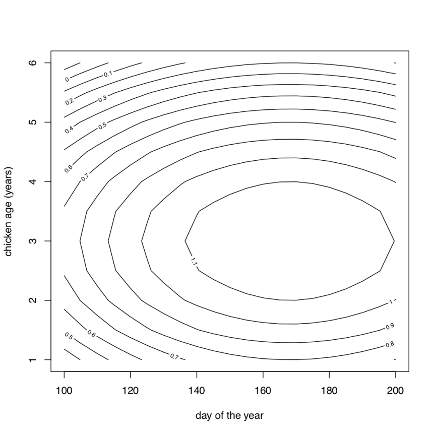

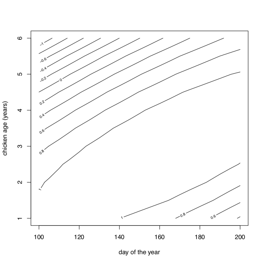
unnamed-chunk-32-1

C8.Q3 If it were to prove that I was basically right, but that additionally as birds get older, their peak of laying gets somewhat later in the year than the solstice, how would the function be different from what you arrived at in the last question?

We need to add a bit of a diagonal ridge shape to our function. If you consider the different shapes plotted in figure 8.7, you should see that what we need is a positive interaction as in figure 8.8a. We need to add a term $\gamma_{ad}(d-168)(a-3)$ to our model. We can try an interaction of $\gamma_{ad}=+0.005$ (something intermediate between the magnitudes of quadratic terms is often a good starting place for an interaction). So our polynomial would look something like:
$eggs = -2.5224 +0.0336 d- 0.0001d^2+0.6a- 0.1a^2$
$~~~~~~~ + 0.005(d-168)(a-3)$
$= -2.5224 +0.0336 d- 0.0001d^2+0.6a- 0.1a^2$
$~~~~~~~ + 0.005(ad - 3d -168a + 3 cdot 168)$
$= -0.0024 +0.0186 d- 0.0001d^2-0.24a - 0.1a^2 + 0.005ad$

Notice that the quadratic terms and the interaction term are the quantities that we originally used for $\gamma_d$ , $\gamma_a$ and $\gamma_{ad}$ . The terms that are harder to make sense of are the linear terms and the intercept, which need to take difficult-to-interpret values in order to place the maximum at the right height (1.2 eggs per day) and at the right values of day of the year and age of the chicken.

# predict egg production on the same range 
# of day of year and chicken age as before
preds$eggs<- -0.0024 +0.0186*preds$d - 
    0.0001*preds$d^2-0.24*preds$a - 
    0.1*preds$a^2 + 0.005*preds$a*preds$d

# plot the expected values of overall height
contour(matrix(preds$eggs,21,11),xaxt='n',yaxt='n',
     xlab="day of the year",ylab="chicken age (years)")
# axes are a bit laborious on contour plots
# but you gotta do it
axis(side=1,at=seq(0,1,length.out=6),
  seq(100,200,by=20))
axis(side=2,at=seq(0,1,length.out=6),
  1:6)

unnamed-chunk-33-1

Share this: